
If there’s one shape that dominates the world of statistics, it’s the bell curve. Officially called the Normal Distribution, this curve is so fundamental that once you recognize it, you’ll start spotting it everywhere — in classrooms, hospitals, stock markets, and even in the quality of the products we buy.
But what exactly is the normal distribution, and why is it so powerful? Let’s take a closer look.
What Is the Normal Distribution?
At its core, the normal distribution is a continuous probability distribution that is perfectly symmetrical around its mean. Imagine plotting test scores from a large classroom: most students would score around the average, while only a few would get very low or very high marks. If you turned that data into a histogram, it would form a familiar bell shape — highest in the middle, tapering off on both sides.
That’s why it’s often called the Gaussian distribution or simply the bell curve.
Key Characteristics
The beauty of the normal distribution lies in its elegance. The center of the curve is not just the mean, but also the median and the mode — all three meet at the same point. The “spread” of the curve depends on the standard deviation (σ). When σ is small, the bell looks narrow and steep, meaning most values are tightly packed around the mean. When σ is large, the bell is flatter and wider, showing more variation in the data.
And here’s something remarkable: the total area under the curve is always equal to 1, representing 100% probability.
The formula that defines this distribution may look intimidating at first glance:
[latex] \frac{x}{y} [/latex]
$$f(x|\mu,\sigma^2) = \frac{1}{\sqrt{2\pi\sigma^2}} e^{ -\frac{(x-\mu)^2}{2\sigma^2} }$$
In this expression, μ represents the mean, σ the standard deviation, and e is Euler’s number (~2.718). Don’t worry if that seems abstract — the formula is simply a way of describing the elegant shape of the bell curve.
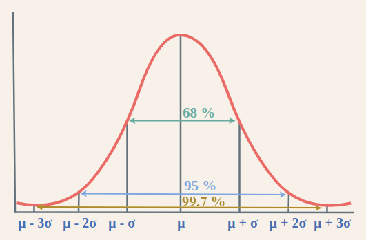
The 68–95–99.7 Rule
One of the reasons the normal distribution is so beloved is because of how predictable it is. Roughly 68% of all data points fall within one standard deviation of the mean. Expand that to two standard deviations, and you cover 95% of the data. Stretch it out to three, and you’ve accounted for 99.7% of observations.
This “68–95–99.7 rule” gives us a quick way to estimate probabilities and set expectations. For example, if exam scores in a school follow a normal distribution, we immediately know that only about 5% of students will score two or more standard deviations away from the average.
Why Does It Matter in Real Life?
The normal distribution isn’t just a mathematical curiosity — it appears everywhere. In education, standardized test scores and IQ results often follow a bell curve. In healthcare, measures like blood pressure, cholesterol levels, or patient recovery times tend to distribute normally. In finance, stock returns and portfolio risks are modeled with normal assumptions. And in manufacturing, quality control depends on detecting when products deviate too far from the expected distribution, a method known as Six Sigma.
In short, whenever there’s natural variation, chances are good that a normal curve is behind it.
Standardization and the Z-Score
Sometimes, working with different normal distributions can get messy. One test may have an average score of 50 with a standard deviation of 10, while another has an average of 500 with a deviation of 100. How do we compare them?
That’s where the Standard Normal Distribution comes in. By converting data into a standardized form where the mean is 0 and the standard deviation is 1, we can compare values across different contexts.
The tool we use for this conversion is the Z-score, calculated as:
$$z = \frac{x – \mu}{\sigma}$$
This tells us how many standard deviations away from the mean a value lies. For example, if a student’s test score has a Z-score of +2, it means they performed two standard deviations above average — placing them well into the top 5% of the group.
Z-scores are not just useful in education. They are critical in hypothesis testing, confidence intervals, outlier detection, and even machine learning, where bringing features onto a common scale (standardization) often improves model performance.
Wrapping It All Together
The normal distribution is far more than a neat mathematical curve. It is the foundation of statistical thinking, giving us the tools to describe uncertainty, compare data across different contexts, and make predictions about the future.
Whether you are a researcher testing a medical treatment, a financial analyst modeling risk, or a data scientist training algorithms, you are relying — often unconsciously — on the power of the bell curve.
So the next time you spot that smooth, symmetrical hump in your data, pause for a moment. You’re looking at one of the most universal and powerful patterns in all of statistics.
Siddharth Singh