
When we first learn regression models, Linear Regression and Logistic Regression often appear side by side. Both are simple, both are widely used, and both rely on similar-looking equations. But when it comes to optimization, they couldn’t be more different.
While linear regression can be solved with a simple formula, logistic regression requires us to rely on gradient-based optimization methods. Why is that the case? Let’s break it down.
Linear Regression: Closed-Form Simplicity
Linear regression predicts continuous outcomes, like house prices or sales figures. Its objective is to minimize the Mean Squared Error (MSE) between predictions and actual values:
[latex]J(\theta) = \frac{1}{2m} \sum_{i=1}^m (y_i – \hat{y}_i)^2[/latex]
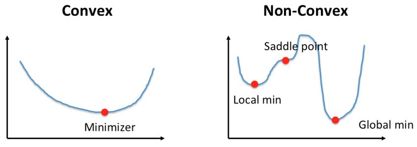
This function is a convex quadratic in the parameters. Because of its convexity and smoothness, we can solve for the parameters directly using the Normal Equation:
$$\theta = (X^TX)^{-1} X^Ty$$
No iteration is needed — the solution “drops out” in closed form.
Logistic Regression: No Closed-Form Solution
Logistic regression, on the other hand, is used for classification problems. Instead of predicting continuous values, it predicts probabilities using the sigmoid function:
$$\hat{y} = \sigma(z) = \frac{1}{1 + e^{-z}}, \quad z = X\theta$$
To estimate parameters, we don’t minimize squared error — we maximize the likelihood of the observed data. In practice, this is equivalent to minimizing the log loss (cross-entropy loss):
$$J(\theta) = -\frac{1}{m} \sum_{i=1}^m \Big[ y_i \log(\hat{y}_i) + (1-y_i)\log(1 – \hat{y}_i) \Big]$$
Here’s the key: this loss function is convex but not quadratic. Unlike in linear regression, there’s no neat formula to solve for $\theta$. The optimization landscape is smooth, but we need to search for the best parameters iteratively.
That’s where gradient-based optimization comes in.
Why Gradient-Based Methods Work
The gradient of the log-loss function tells us the direction in which we should adjust the parameters to reduce error. Optimization algorithms like Gradient Descent update parameters iteratively until convergence:
$$\theta := \theta – \alpha \nabla J(\theta)$$
where alpha is the learning rate.
This process allows us to efficiently minimize the loss, even though no closed-form solution exists.
Optimizers in Scikit-learn
Scikit-learn’s LogisticRegression does not use vanilla gradient descent by default. Instead, it provides several solvers (optimizers), each with its own strengths:
- liblinear – A coordinate descent algorithm. Best for small datasets and binary classification.
- lbfgs – An approximation of Newton’s method. Handles multiclass problems well and is efficient for medium-sized datasets.
- newton-cg – Newton-Raphson based optimizer. Good for multiclass, slower but accurate.
- sag (Stochastic Average Gradient) – Designed for large datasets, updates parameters using mini-batches.
- saga – An extension of SAG, supports L1 regularization and is more robust.
In practice, lbfgs and saga are the most widely recommended, especially for large-scale or regularized logistic regression.
Why Not SGD?
At this point, you might wonder: why can’t we just use Stochastic Gradient Descent (SGD)? After all, it’s the simplest gradient-based optimizer.
The problem lies in the nature of the logistic loss function:
- Logistic regression loss is smooth but relatively flat near the optimum. SGD, with its noisy updates, may wander around instead of converging precisely.
- SGD requires careful tuning of the learning rate and often converges much slower compared to second-order methods like lbfgs.
- Regularization (L1 or L2) adds another layer of complexity that basic SGD doesn’t handle well.
For these reasons, scikit-learn implements more advanced solvers that provide faster convergence, better stability, and built-in support for regularization.
Wrapping Up
The difference between linear and logistic regression isn’t just about predicting numbers vs probabilities. It’s also about how we find the parameters that make the model work.
- Linear regression → closed-form solution, no need for gradient optimization.
- Logistic regression → no closed-form solution, requires iterative optimization.
- Scikit-learn solvers → from liblinear to lbfgs, provide efficient ways to minimize log-loss.
- Why not SGD? → too unstable and inefficient for logistic regression’s convex but tricky landscape.
So the next time you run LogisticRegression in scikit-learn, remember: behind that simple .fit() call, a powerful optimization engine is working hard to find the parameters — one gradient step at a time.